31 Dec

How To Find Last Occurrence of Character in a String

There may be some instances where you will need to find the last occurrence of a specific character in a string in Excel. The following example shows you how.

Assuming that your original string is in cell B2 and the character that you want to find is “.” , the formula to give you the position of the last occurrence of the character in the string is:
=LEN(B2)-LEN(TRIM(RIGHT(SUBSTITUTE(B2,”.”,REPT(” “,LEN(B2))),LEN(B2))))

The following shows a breakdown of the above formula:

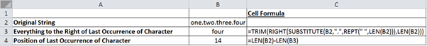
The key to this example is this magical formula, which gives you everything to the right of the last occurrence of the character “.”.
=TRIM(RIGHT(SUBSTITUTE(B2,”.”,REPT(” “,LEN(B2))),LEN(B2)))

Let me know if you need more explanation of the above. Thanks!

15 Dec

How To Shorten Number Formats with Millions or Thousands

When we have large numbers, we often want to use the contraction “K” or “M” for thousands or millions respectively. To do this in Excel, we need to change the number format to the following.

For thousands (and 2 decimal places):
0.00,”K”
[1,234 is shown as 1.23K]

For millions (and 2 decimal places):
0.00,,”M”
[1,234,567 is shown as 1.23M]

One good use of number formats is in charts, as seen below. This uses the format 0,,”M” in the vertical axis and the format 0.00,,”M” in the data labels.

The above is based on a very good reference on number formats from Peltier Tech (http://peltiertech.com/Excel/NumberFormats.html) which has detailed explanations and as many things as you can think of to do with number formats!

The site also provides a conditional number format – where numbers greater than 1 million are shown with an “M”, and numbers greater than 1 thousand are shown with a “K”.

[>=1000000]0,,”M”;[>=1000]0,”K”;0